Die diskrete Fourier-Transformation (DFT)

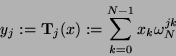
Definition 1 (DFT)      Die diskrete Fourier-Transformation (DFT) der Länge N ist gegeben durch

$$\mathbf{T}: {\mathbf{C}}^N \to {\mathbf{C}}^N,$$

$$y_j := \mathbf{T}_j(x) := \sum_{k=0}^{N-1} x_k \omega_N^{jk}$$ (1)

mit

$$\omega_N := e^{\frac{-2 \pi i}{N}} = \cos(2\pi/N) - i \sin(2\pi/N).$$ (2)

In der Definition läßt sich direkt ablesen, daß jeder Ergebniswert $y_j$ von allen Eingangswerten $x_k$ abhängt. Ein naiver iterativer Algorithmus zur Berechnung der DFT hat also eine Zeitkomplexität von $O(N^2)$.

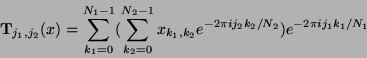
Definition 2 (2D-DFT)      Die 2D-DFT ist gegeben durch

$$\mathbf{T}: {\mathbf{C}}^{N_1 \times N_2} \to {\mathbf{C}}^{N_1 \times N_2},$$

$$y_{j_1, j_2} := \mathbf{T}_{j_1, j_2}(x) := \sum_{k_1=0}^{N_... ...^{N_2-1} x_{k_1, k_2} e^{-2\pi i (j_1 k_1/N_1 + j_2 k_2/N_2)}.$$ (3)

Die 2D-DFT läßt sich auf die 1D-DFT zurückführen

$$\mathbf{T}_{j_1, j_2}(x) = \sum_{k_1=0}^{N_1-1} ( \sum_{k_2=... ...x_{k_1, k_2} e^{-2\pi i j_2 k_2/N_2} ) e^{-2\pi i j_1 k_1/N_1}$$ (4)

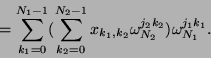$$= \sum_{k_1=0}^{N_1-1} ( \sum_{k_2=0}^{N_2-1} x_{k_1, k_2} \omega_{N_2}^{j_2 k_2} ) \omega_{N_1}^{j_1 k_1}.$$ (5)